Waiting to Get Your Dissertation Accepted?


Binary logistic regression is a very useful statistical tool, under the right circumstances. But, it requires a bit more understanding and effort to interpret the results than other tools in the same family. In this article, I’ll show you how to execute a binary logistic regression analysis and interpret its results. These are the essentials—what you need to know to perform a binary logistic regression analysis for a thesis or dissertation.
Binary Logistic Regression—When & Why?
Often, in statistical analysis including academic theses and dissertations, we are predicting an outcome (response or dependent variable) based on the values of a set of predictors (categorical factors or numerical independent variables).
The most common tools to do this are regression analysis and analysis of variance (ANOVA). In these analyses, we are trying to predict a numerical dependent variable—something that we can count or measure, like hardness of steel or the number of people with a certain attribute.

Sometimes, though, we are interested in a binary dependent variable—the outcome has two values, such as yes or no. In the medical field, for example, we might predict whether a treatment will be successful or unsuccessful.
For these cases, ANOVA and linear regression are not suitable tools, because they require a numerical dependent variable. But, fortunately, there is binary logistic regression. This tool enables us to predict the likelihood of a binary outcome as a function of the values of our predictors.
But First—A Caution!
If you have a numerical dependent variable, either measured or counted, you should use it!
Often, I see students and analysts converting perfectly valid numerical variables into categorical or binary outcomes. This is not a good idea.
Let’s say we are interested in the mileage of vehicles, based on several postulated control factors (e.g., percentage of ethanol in the gasoline). We have a perfect setup for multiple linear regression, with measurable independent variables and a dependent variable. But, there is this urge for analysts to convert measured mileage to categories: extremely high, high, medium, low, and extremely low mileage. Why???

By doing this, we lose a significant amount of information from the precise measurement of mileage in each trial to a fuzzed-up set of categories, with a loss of statistical power and confidence. And, it could be worse, if we converted our measurable, numerical dependent variable to a binary outcome: high and low mileage.
This is a cardinal sin in statistical analysis. Use categorical variables only when they are unavoidable (non-measurable traits, or outcomes that can only be characterized by a yes or no response).
Some Concepts and Definitions
The dependent variable in binary logistic regression is dichotomous—only two possible outcomes, like yes or no, which we convert to 1 or 0 for analysis. It is either one or the other, there are no other possibilities.
Get Your Dissertation Accepted On Your Next Submission

Odds

At the heart of binary logistic regression are two concepts related to the binary outcomes. The first is the concept of odds: How much more likely one outcome is over another outcome. Or, more precisely, the ratio of the probability that outcome #1 will occur to the probability of outcome #2. Mathematically . . .
odds = p1/1-p1 = p1/p2 where p1 is the probability of outcome #1, and
1 – p1 = p2 is the probability of outcome #2.
Note that there are only two outcomes, so the probability of one plus the probability of the other equals 1. And, if outcome #1 and outcome #2 are equally likely, then p1 = p2 = .50, and the odds are 1 to 1 (i.e., “even odds” or “50-50”).
The “Logit”
The second concept is the logit, the natural logarithm of the odds of outcome #1:
logit = Li=ln[p1/(1-p1)]
This concept is a bit less intuitive than odds, but suffice to say that transforming the dependent variable (i.e., converting a dichotomous dependent variable [0 or 1] or odds to a natural logarithm) enables us to overcome the requirement of linearity between independent variables and the dependent variable required in conventional regression.
Binary Logistic Regression vs. Linear Regression

Now, let’s talk about how binary logistic regression is different from linear regression. In linear regression, the idea is to predict the value of a numerical dependent variable, Y, based on a set of predictors (independent variables). In general terms, a regression equation is expressed as
Y = B0 + B1X1 + . . . + BKXK where each Xi is a predictor and each Bi is the regression coefficient.
Remember that for binary logistic regression, the dependent variable is a dichotomous (binary) variable, coded 0 or 1. So, we express the regression model in terms of the logit instead of Y:
logit = Li = B0 + B1X1 + . . . + BKXK
Assumptions of Binary Logistic Regression
Next, let’s quickly review the assumptions that must be met to use binary logistic regression. All statistical tools have assumptions that must be met for the tool to be valid for our analysis. One advantage of binary logistic regression is that it enables us to overcome some of the assumptions required in linear regression and ANOVA.

Here are the assumptions for binary logistic regression:
- The dependent variable is measured on a dichotomous scale (only two nominal/categorical values).
- The dependent variable has mutually exclusive and exhaustive categories/values.
- One or more numerical independent variables.
- Independence of observations.
- A linear relationship between the numerical independent variables and the logit transformation of the dependent variable.
Binary Logistic Regression: Questions and Analysis
There are several pieces of information we wish to obtain and interpret from a binary logistic regression analysis:
- What is the best predictive model (set of independent variables) of the logit?
- Is the model of predictors significant compared to a constant-only or null model?
- What are the predictors which comprise the final and best predictive model?
- What is the strength of the association between the independent variables and the dependent variable?
- What is the interpretation of the coefficients (Bs) and Exp(B)?
- Given values for the predictors, what is the predicted value of the dependent variable?

Illustration of Binary Logistic Regression
Here is an illustration of binary logistic regression and the analysis required to answer these questions, using SPSS as the statistical workhorse. The example (SUV ownership) is based on an available data set, where
Y = OwnSUV (a categorical dependent variable with values: 1 = yes, 0 = no)
X1 = age (a numerical independent variable)
X2 = respondent’s gender (categorical independent variable with values: 1 = male, 0 = female)
The analysis can be done with just three tables from a standard binary logistic regression analysis in SPSS.
Step 1. In SPSS, select the variables and run the binary logistic regression analysis. Evaluate the significance of the full model using the Omnibus Tests of Model Coefficients table:
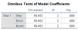
In this table, 𝜒2 = 50.452, p = .000. We conclude that the full model is significantly different from a constant-only or null model (even odds); therefore, the model is a significant predictor of the dependent variable.
Step 2. Evaluate the strength of the association between the model (all independent variables) and the dependent variable using the Model Summary table:
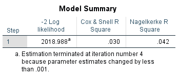
The strength of the association between the model composed of two independent variables and the dependent variable (the strength of the model, or goodness-of-fit) is based on *Nagelkerke’s R2 = .042. Only 4.2% of the variation in the dependent variable is attributed to the model. We conclude that while the model is a significant predictor of the dependent variable, it is likely there are other independent variables that may be significant predictors.
[*I used Nagelkerke’s R2 because it is normalized to produce values between 0 and 1, as in R2 used in conventional regression analysis.]
Step 3. Evaluate the strength of the association between each independent variable and the dependent variable using the Variables in the Equation table:
Variables in the Equation
| B | S.E. | Wald | df | Sig. | Exp(B) | |||
| Step 1a | Age of respondent | .016 | .003 | 26.711 | 1 | .000 | 1.016 | |
| Respondent’s Gender | .530 | .107 | 24.350 | 1 | .000 | 1.698 | ||
| Constant | -1.791 | .174 | 105.672 | 1 | .000 | .167 |
We use the Wald ratio for each of the independent variables and its associated p value:
𝜒2(1) = 26.711, p = .000; and 𝜒2(1) = 24.350, p = .000 respectively. We conclude that the coefficients for both of the independent variables are significantly different from those in the even odds (null) model; therefore, these independent variables are significant predictors of the dependent variable.
Step 4. Remembering that the dependent variable is a dichotomous (binary) variable, coded 0 or 1, we express the predictive regression equation using the coefficients from the Variables in the Equation table:
Li=B0+B1X1+B2X2=(-1.791)+0.016X1+0.530X2
Step 5. Interpretation of the coefficients (from the Variables in the Equation table):
The logit increases (or decreases) by Bi for a unit increase in predictor, Xi. This can be illustrated with nominal values for the independent variables (see step 6).
Exp(B) indicates the change in predicted odds of the outcome (in this case, SUV ownership) for a unit increase in the predictor.
For age, the odds of SUV ownership increase by a factor of 1.016 for each year increase in age.
For gender, SUV ownership increases by a factor of 1.698 for males versus females. Males are 1.698 more likely than females to own a SUV.

Step 6. Finally, given any set of values for the predictors, Xi, calculate Li and convert that into odds to predict the probability of membership in the target group (SUV ownership). This can be done by using this formula, which is then illustrated with the example to follow:
Pi=eLi/1+eLi
Interpretation of Binary Logistic Regression: An Example
Let’s work through our example, with some values for the independent variables, to show how to interpret a binary logistic regression analysis.
For a male (X2 = 1) of 30 years (X1 = 30),
Li = (−1.791) + (.016)∙(30) + (0.530)∙(1) = −.781
eLi = 0.458
p1 = 0.458 ÷ (1 + 0.458) = .314
The probability of a 30-year-old male owning a SUV is .314, or 31.4%. This is a conditional probability because it is the probability of one outcome (SUV ownership) given two other conditions (specific values for gender and age).
The odds of a 30-year-old male owning a SUV
= p1/(1-p1) = .314 ÷ (1 − .314) = 0.458
Similarly, for a 30-year-old female (X2 = 0):
Li = (−1.791) + (.016)∙(30) + (0.530)∙(0) = −1.311
eLi = 0.270
p2 = 0.270 ÷ (1 + 0.270) = .212
The probability of a 30-year-old female owning a SUV is .212, or 21.2%. This is a conditional probability because it is the probability of one outcome (SUV ownership) given two other conditions (specific values for gender and age).
The odds of a 30-year-old female owning a SUV
= p2/(1-p2) = .212 ÷ (1 − .212) = 0.270
Males are 1.698 times more likely to own a SUV than females (0.458 ÷ 0.270).
If age (X1) increases by one year, the regression model and coefficient for age (0.016) predicts that the logit (Li) increases by 0.16, all other variables remaining constant.
For a 60-year-old male,
Li = (−1.791) + (.016)∙(60) + (0.530)∙(1) = −0.301

eLi = 0.740
p1 = 0.740 ÷ (1 + 0.740) = .425
Note that for a 30-year increase in age, Li changes by 30∙(0.16) = 0.480. In fact, Li changed from −0.781 (age = 30) to −0.301 (age = 60), an increase of 0.480. The probability changed from .314 to .425.
Conclusion
The example illustrates all the useful information we can derive from a properly executed binary logistic regression analysis.
Binary logistic regression is an often-necessary statistical tool, when the outcome to be predicted is binary. It is a bit more challenging to interpret than ANOVA and linear regression. But, by following the process, using only what you need from SPSS, and interpreting the outcomes in a step-by-step manner using the formulas, you can obtain some useful and understandable information.