Waiting to Get Your Dissertation Accepted?


Among the most important components of multi-variate analysis and model-building (e.g., multiple regression and ANOVA) are two-factor interactions (or, 2-factor interactions). 2-factor interactions provide some of the most insightful outcomes of analysis in dissertations, theses, and practical applications.
The concept of 2-factor interactions is a bit challenging to understand at first. But, in this article, I will explain what they mean and how to identify them. And, most importantly, how to interpret 2-factor interactions.
Two-factor Interactions: What are they?
First: A review of multi-variate analysis

We are often interested in learning about some measurable, real-world phenomenon. It might be a human behavior, such as demand for a product (e.g., gasoline) or a scientific phenomenon (e.g., blood pressure), which can be counted or measured as response variables, Y.
We postulate that these response variables are influenced by, predicted by, associated with, or caused by some set of predictors (factors or independent variables)—call these A, B, C, and so on; or, in math terms: X1, X2, X3, . . . .
For example, blood pressure (Y) might be predicted as a function of age, body mass index, smoking, family history, medicine, and physical activity (A, B, C, . . .).
But, here is the issue. The real-world is complicated! And, blood pressure is a complex phenomenon!. Various factors cause or influence blood pressure in varying degrees, and interact with each other in different combinations.
So, what is a 2-factor interaction?
We might find that A is associated with Y. But, the relationship of A to Y depends on the value of another predictor, B. Note in the figure below:
- When B is low, the relationship between Y and A is linear and negative.
- When B is at its average value, the relationship between Y and A is now positive.
- And, when B is high, the relationship between Y and A is even more steeply positive.
- Probably, at some value of B, the line is flat—no slope, no influence on Y.
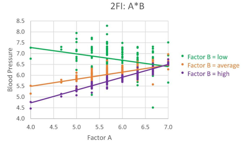
The 2-factor interaction called A*B tells us that the relationship between Y and A depends on the value of B. We also say that B is a moderating variable, because it moderates the influence of A on Y.
Why are 2-factor interactions important?
The presence of a significant 2-factor interaction means that we cannot make blanket, generalized, unqualified statements about the influence of A on Y. That influence, or relationship, changes; and it depends on factor B.
Get Your Dissertation Accepted On Your Next Submission

In our notional example, the effectiveness of the dosage of medicine (captured in A) depends on age (factor B):
- For younger people, the medicine’s effect decreases as the dosage increases.
- But, for people of average to high age, the medicine’s effect increases with dosage.
- And, at some age, the medicine’s effectiveness likely does not change with dosage.
You can see that the 2-factor interaction is eminently important. Because without it, our claims about A and Y are incomplete and flawed. And, without considering the 2-factor interaction, we might make a bad conclusion about the influence of A, and perhaps a bad decision regarding people’s health.
How do we identify 2-factor interactions?
A review of regression and ANOVA
Let’s start with this: We employ multi-variate analysis to learn the following:
- Which independent variables are significant predictors of the response variable?
- Which exert no significant influence on the response?
- What is the best possible predictive model (set of predictors including 2-factor interactions)?
- What is the sensitivity of the response to each of the predictors?
To address these questions, we develop the best predictive model of Y based on a data set. And, the predictors that comprise that model, along with their coefficients, provide the answers. That model is expressed in a mathematical equation:
- Y^ = b0 + b1X1 + … + bkXk
where
- Y^ (“Y-hat”) is the predicted value of the response variable
- Xj is the jth predictor of Y (and might be a 2-factor interaction such as Xa ∙ Xb)
- b0 is the value of Y when all predictors equal zero
- bj is the coefficient for the predictor, Xj (a measure of its influence).
Mathematically, 2-factor interactions are the product of each pair of independent variables. For example, if A = X1 and B = X2, then the 2-factor interaction we call A*B is equal to X1 ∙ X2. We compute these 2-factor interactions in our data set in Excel, by creating new columns for each 2-factor interaction. The value is the product of the two predictors (columns) that comprise the 2-factor interaction.
A review of model-building

A proper application of multi-variate analysis—to find the best predictive model—requires model-building. A one-time run of regression analysis or ANOVA with independent variables is incomplete. But, why?
Most real-world phenomena—including those studied in graduate-level analysis—are incompletely understood, especially their causes or influences (that’s why we study them!). Predictive model-building assists in making sense of the data and closing the information gap.
There may be many causes of a phenomenon, and they may interact among themselves. For example, there are many factors influencing grade point average (including, for example, age, family income, location, gender). The relationship between age and grade point average may change depending on gender—a classic 2-factor interaction.
In reality, there may be many interactions among causes—some very small, subtle, unknown, and perhaps unmeasurable. But, collectively these interactions are enough to cause variation in the response that is difficult to explain.
On the other hand, some interactions are likely, known, observable, and perhaps measurable or capable of being calculated. Even when the predictors are controlled and measured, and the response is measured precisely, there is inevitably some variation in the response for reasons that may be unknown—it may be that the process is simply noisy, and there is no scientific explanation for that noise.
In our zeal to find predictors and causes, we inevitably learn that the influence of a predictor depends on the presence of other predictors in the predictive model. Again, this is because real-world phenomena are complex, with many interdependencies and interactions among causes and influences.
Some predictors influence the response, but not directly—sometimes as a moderator of another factor. Or, sometimes because the true predictor is really a combination of two factors, not a factor by itself. We learn this only through model-building.
So, failing to account for the complexity, the interactions, and the interdependencies among causes may mask the true influence of a single factor.
We simply cannot make a truthful statement about the influence of any predictor without simultaneously considering all of the influential factors that we know about, or that we can find. And, these are expressed in our mathematical model. And, that model is developed through a rigorous model-building process.
With this mathematical model (and the analysis used to develop it), we can determine the influence of various predictors. We start with all of the predictors we postulate are associated with Y, and use analysis and model-building to determine which should be included in the predictive model. Those that make the cut, including the 2-factor interactions, are what we conclude are the (likely) true predictors of the response. Not because they are evaluated separately, but precisely because they are evaluated as part of the whole model—considering the interdependencies among them all.
Model-building to identify 2-factor interactions

Imagine if we have a problem for which there are many possible predictors of a phenomenon (a response). And, if we concede that there may be interactions between these predictors, then it is easy to see how complex the analysis might get.
Say we have a complex real-world problem that is poorly understood, but our smart subject matter experts identify 10 “likely” predictors. If we do the right thing and assess the 2-factor interactions, we have a big math problem. There would be 45 2-factor interactions to evaluate, and a pretty hefty challenge for our computers and software.
A good way to handle this challenge is what we call a sequential approach to model building. Model-building is performed in four stages:
- Stage 1: Identify candidate predictors based on theory, previous research, empirical results, and subject matter expertise (SME).
- Stage 2: Screening. Employ regression or ANOVA to identify and eliminate candidates that are highly likely NOT to be significant predictors of the response variable.
- Stage 3: Compute the 2-factor interactions from the remaining candidate predictors. Perhaps we have six predictors remaining, which then would generate 15 2-factor interactions.
- In Stage 4, we employ various regression techniques, to analyze remaining independent variables and 2-factor interactions, and to select the final predictive model (eliminating non-significant predictors).
Model-building employs several regression techniques (collaboratively and iteratively) to select the predictors that comprise the final and best predictive model of the response variable. The techniques include best-subsets regression, purposeful sequential regression, and statistical regression. We employ all regression techniques to generate statistical evidence to select the best predictive model, while overcoming the deficiencies of any one technique. I plan to explain the model-building process and the use of more than one regression technique in another article.
We also rely on SMEs, analyst judgment, and some trial-and-error—trying various combinations of techniques and models. We are continuously striving to improve the goodness-of-fit (based on adjusted R2 and Mallow’s CP statistic). This process continues until the model is predicting as well as possible, with terms that make sense.
Interpreting 2-factor interactions

How We Analyze the 2-factor interactions
Powerful apps such as SPSS can help to build graphical depictions of 2-factor interactions. I prefer to build them in Excel, as I did for the figure shown earlier. I will devote another article on how to do this. In any case, we are building scatterplots with trend lines to show relationships between predictors and the response.
In our example, as with any 2-factor interaction, there are two axes (vertical axis is Y, horizontal axis is predictor A), and three unique sets of data points with trendlines. The three data subsets reflect three values of the second predictor in the 2-factor interaction (in this case, B). The trendlines show the relationship between Y and A when B is at its minimum, its average, and its maximum.
If the 2-factor interaction was found to be significant in Stage 4 of the model-building process (and if not, it would not be in the final model), the lines will be non-parallel. This indicates visually that the relationship between Y and A changes as B changes value. Incidentally, we can and should depict the 2-factor interaction reflecting the relationship between Y and B, for different values of A.
As we discussed earlier, there is a significant 2-factor interaction (A*B) found in the analysis (based on a t test), and the earlier figure shows that the trendlines are not parallel, confirming the 2-factor interaction. We are able to see visually that the effectiveness of the dosage of medicine (captured in A) depends on age (factor B)—i.e., the relationship changes as the value of B changes.
By the way, here is a depiction of Y versus factor A, for all values of B. Note that, overall, Y increases with increases in A.
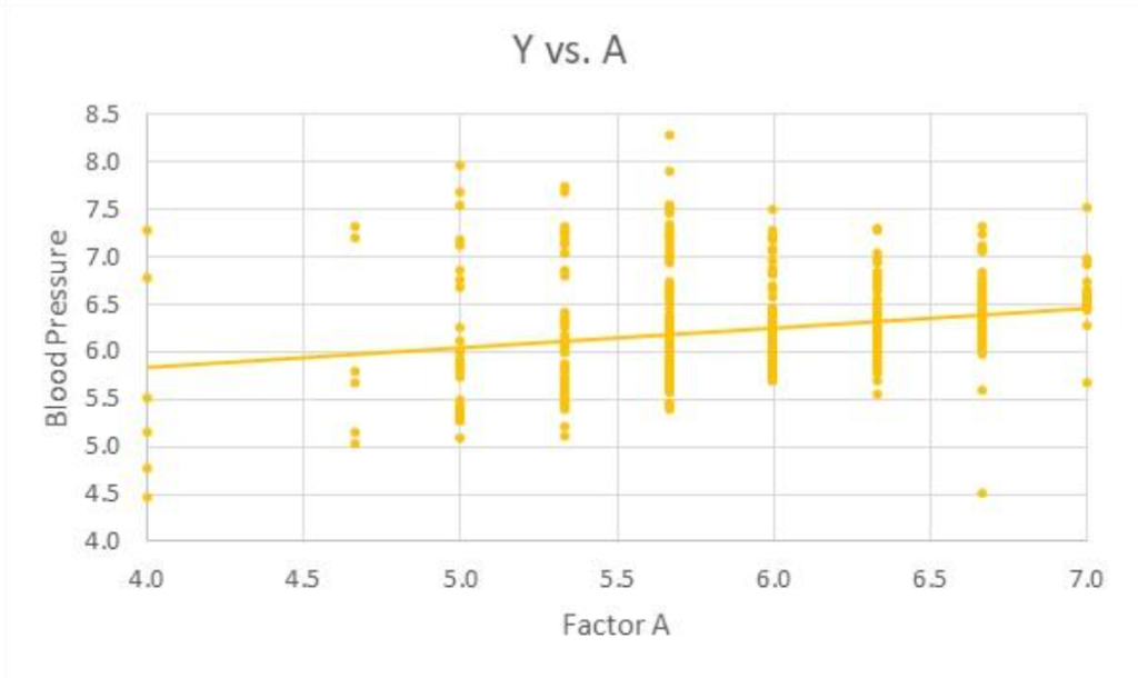
But, the important conclusion here in our analysis is this: It is not accurate to say that Y increases with A even though the coefficient of A in the regression equation is positive (as shown in the figure). It is true that, all other factors being constant, that Y increases by an amount equal to A’s coefficient for each unit increase in A.

But, the 2-factor interaction indicates that the claim (of a main effect of A on Y) depends on the value of another predictor, B. Not only, in this case, does the amount change by which Y increases as a function of A depending on B (the magnitude of the coefficient), but the direction changes as well, which is a really significant finding. This illustrates the importance of including 2-factor interactions in the predictive model and explaining the influence the interaction has on the predictive model.
What the 2-factor interactions might mean
Once we have discovered significant 2-factor interactions, and have looked over their graphical depictions, we may find a few different situations:
- Situation 1 is a 2-factor interaction involving two significant independent variables. Both are significant predictors of the response. But, in addition, the influence of each is moderated by the other predictor—their influence is a combination of both.
- In situation 2, a predictor B might not be a significant influence on Y by itself, but it exerts a moderating effect on another predictor of Y (A)—on the relationship between Y and A. B is not significant by itself, but a moderator of A.
- In situation 3, two independent variables are not significant by themselves, but in combination they exert a significant influence on Y. You might say, there is a new variable whose value is a combination of A and B. And, this new variable exerts an influence on Y.
We find these nuances only by a rigorous model-building process, in stages, with collaborative and iterative, trial-and-error analysis. And, we explain them using subject matter expertise.
Final thoughts
There is always a need to go beyond simply reporting the statistical results. The researcher or analyst must also explain . . .
- how the statistical results are explained and interpreted
- what the statistical results are saying about the real-world phenomenon
- what the statistics are revealing about what is really going on, from an operational or practical perspective.
It may require consulting with a subject matter expert to explain why some predictors in our final predictive model are included and others are not. But, what we have shown in this article goes even farther—explaining why the influence of a predictor may be moderated by another predictor. And, that only can occur if we include 2-factor interactions in our analysis and interpretation.
References
IBM Corporation. (2020). IBM SPSS Statistics for Windows, Version 27.0. Armonk, NY: IBM Corp.
Levine, D. M., Berenson, M. L., Krehbiel, T. C., & Stephan, D. F. (2011). Statistics for managers using MS Excel. Boston, MA: Prentice Hall/Pearson.
Warner, R. M. (2013). Applied statistics: From bivariate through multivariate techniques. Los Angeles: Sage.