Waiting to Get Your Dissertation Accepted?


Another technique in your toolkit of multi-variate analyses is analysis of variance (ANOVA).
In this article, I describe ANOVA, contrast it with regression, and tell you what you need to know to execute the technique properly for your theses, dissertations, and real-world analyses.
What is ANOVA?
Univariate ANOVA is used to determine the relationship between categorical predictor variables—often called control factors—and a single numerical dependent variable. Properly executed, ANOVA yields a predictive model of the dependent variable.
One-way ANOVA evaluates a single predictor with multiple levels (values) and a single dependent variable. Two-way ANOVA evaluates two predictors and a single dependent variable. There is no limit to the number of predictors or their levels that can be analyzed using ANOVA.
ANOVA is often, but not always, used as the analytical tool for designed, factorial experiments. All combinations of the factor levels (cases) are examined, systematically and in equal numbers, to assess the influence that each factor has on the dependent variable.
How do ANOVA and regression compare?

A review of my article on regression will show how similar these techniques are. They’re both powerful tools for evaluating multiple predictors of a phenomenon. They’re different, but they are more common than you might think.
Different statistical models
Regression is used to predict a numerical outcome as a function of one or more numerical predictor variables. ANOVA is likewise used to predict a numerical outcome, but based on one or more categorical predictor variables.
So, if you are trying to predict student achievement test scores as a function of household income and teacher years of experience, then multiple linear regression is the tool. For the same dependent variable . . . predicting achievement test scores based on geographical region and curriculum, use ANOVA. We’ll follow this example through this article.
One other situation: you are predicting test scores based on household income (numerical predictor) and curriculum (categorical predictor)—use regression. Here, you would convert the categorical predictor with two values to a single dummy variable.
Similarities
Both techniques employ similar components, covered in the regression article.
- Both require a numerical dependent variable (discrete or continuous).
- Both use the least squares method, part of the general linear model.
- Both use model-building to find the best combination of predictors and their two-factor interactions. The predictors that comprise the best model are considered significant predictors of the dependent variable.
- The mathematical model-building process relies on the purposeful sequential regression technique.
- They share some of the same mathematical assumptions. I cover those later.
Predictive ANOVA model

The true, theoretical model for a two-way ANOVA (two predictors, A and B) is the following:
Yijk = μY + αi + βj + αβij + εijk.
where
Yijk = value of the dependent variable for record k within the group that corresponds to level i of factor A and level j for factor B
μY = population grand mean of Y values
αi = effect of the ith level of factor A
βj = effect of the jth level of factor B
αβij = interaction effect for the i, j cell (interaction between factors A and B)
εij = unexplained portion of the kth value of Y (i.e., not accounted for in the other terms of the ANOVA equation).
Note that the two-way ANOVA model can be expanded for any number of treatments/factors/predictors (A, B, C, . . .) and their interaction terms.
The final, predictive, ANOVA model is
Y^ijk = μY + αi + βj + αβij
where Y^ijk (Y-hat) is the predicted value of the dependent variable for the kth record.
The equation says, the value of Y for any record (any case, or combination of values for the factors) is predicted to be the sum of the grand mean; the effects of factors A, B, etc.; and the interaction between A and B.
The coefficients in the predictive equation represent the estimated effects (such as αi, the effect of the ith value of factor A) in the ANOVA model.
The difference between the actual value of Yijk and the estimated or predicted value (Yijk,) is the error term, or the residual, for the kth record.
Get Your Dissertation Accepted On Your Next Submission

ANOVA Hypotheses
There are three hypothesis tests in a two-way ANOVA. When evaluating more than two factors, the number of hypotheses increases accordingly.
The hypothesis of no difference in the dependent variable due to factor A:
H0: μ1 = μ2 = ⋯ = μi ⋯ = μm (means for all levels of A are equal)
where the number of levels of factor A = m
against the alternative:
H1: not all μi are equal.
The hypothesis of no difference in the dependent variable due to factor B (which, as an example, has two levels):
H0: μ1 = μ2 (means for both levels of B are equal)
where the number of levels of factor B = 2
against the alternative:
H1: μ1 ≠ μ2 (general form: not all μi are equal).
The hypothesis of no interaction of factors A and B:
H0: the interaction of A and B is equal to zero.
against the alternative:
H1: the interaction of A and B is not equal to zero
Hypotheses are tested using the F test (and its p value). The F test assesses whether a factor predicts the dependent variable (dependent variable means are different for various treatments). Adjusted R2, the coefficient of determination, indicates the extent to which the predictors as a group (model) contribute to the variance in the dependent variable.
ANOVA assumptions

ANOVA assumes the following:
- The dependent variable is a continuous, numerical variable.
- Each predictor consists of two or more categorical and independent groups.
- Independence of observations: no time-related relationship between observations (best defense is randomized data collection; checked with a scatterplot of the dependent variable over time).
- No influential cases: no significant outliers (checked in Excel; one rule of thumb is any value of the dependent variable more than three standard deviations from its mean).
- Experimental errors (residuals) are approximately normally distributed (normal probability plot).
- Homogeneity of variance for each combination of groups/levels/values (Levene’s test).
Factorial ANOVA
A factorial or balanced design is an experiment in which the predictors are crossed: every level of each factor is paired with every level of the other predictors. All cases are examined in equal numbers, to assess the influence of each factor. Controlled experiments use factorial designs with randomization of the cases; and with multiple trials of each case (replication) for adequate sample size. In observations or with secondary data, we often settle for the data we have or can get, and the data set may not be a factorial design.
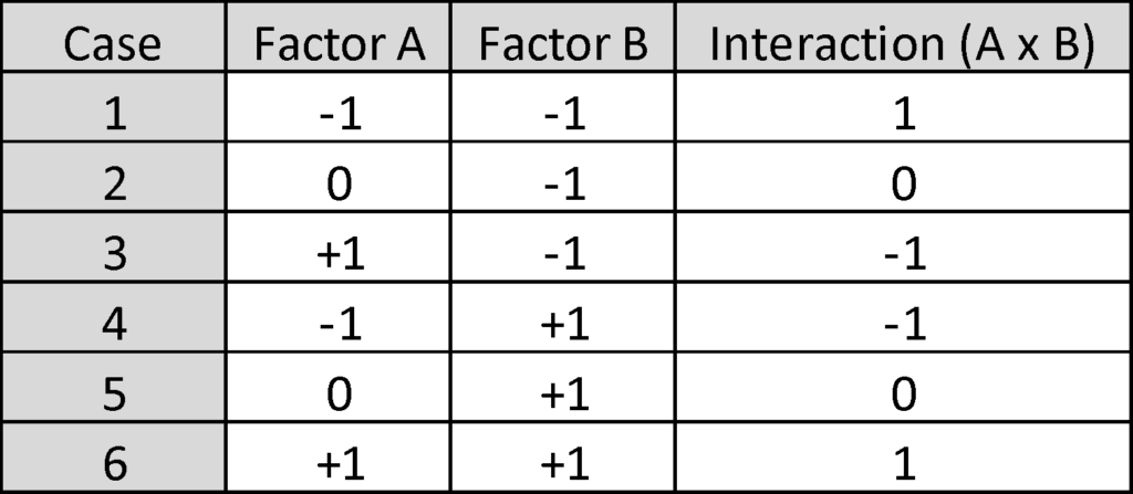
Here is the factorial design for our evaluation of achievement test scores. Factor A (region) has three levels (north, central, south). Factor B (curriculum) has two levels (original and new).
There are 3 × 2 = 6 cases. The factors are categorical variables. But, they are coded to perform the ANOVA algorithm. Mathematically, factor interactions are calculated as the cross-product of values for each factor in the interaction.
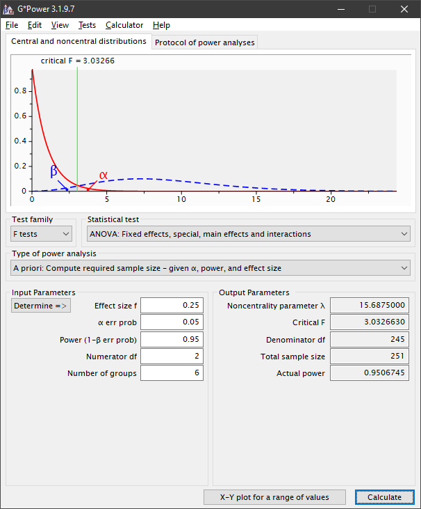
Sample size for ANOVA
Total sample size (n) is the number of cases multiplied by the replicates per case. How many replicates is determined using an app, such as G*Power (Faul et al., 2009). In our example:
- Tests (top menu): Means / Many groups: ANOVA: Main effects and interactions (two or more independent variables); or, Test Family: F tests
- Statistical test: ANOVA: Fixed effects, special, main effects and interactions
- Type of power analysis: A priori: Compute required sample size given α, power, and effect size
- Effect size f (Cohen, 1988): .10 (small), .25 (medium), .40 (large)
- α = .05 (or analyst justified choice)
- Power (1 – β) = .95 (or analyst justified choice)
- Numerator df = number of factor levels – 1 (e.g., factor with most levels is A with 3 levels => numerator df = 3 – 1 = 2)
- Number of groups = product of number of levels for each independent variable (e.g., two factors [A, B] with 3 and 2 levels respectively => number of groups = 3 × 2 = 6)
- Total minimum required sample size = 251
Adjust sample size to ensure equal numbers in each cell (for each group). For example . . .
- Total [minimum] sample size [given specified α, power, and effect size] = 251
- Total number of groups = 6
- Sample size per group = 251 ÷ 6 = 41.8
- Round up to next whole number = 42 = true minimum number per group = replication
- Adjusted total sample size = number of groups × replication = 6 × 42 = 252
Setting up ANOVA in SPSS
First, create a spreadsheet in Excel mirroring the case matrix, with rows for each replication (each data record). Handle missing data or outliers in the data set.
Copy all cells from Excel; then paste to a new data sheet in SPSS (right click on cell A1 and choose “Paste with Variable Names.”).
Set up the problem in SPSS:
- General Linear Model > Univariate (only one dependent variable).
- Select the numerical dependent variable (response) and the categorical factors (predictors). Because ANOVA’s predictors are categorical, designate them as fixed factors.
- Model: “Full factorial”; Sum of squares: Type III; include intercept in model. Or, “Build terms” when the dataset is unbalanced, a particular subset of factors will be evaluated, or when interactions will not be assessed.
- Sum of squares: Type III (because the intent always is to investigate the significance of factor interactions; when factor interactions will not be evaluated, use Type II).
- Contrasts: none.
- Plots: choose one factor for a separate line; and another for the horizontal axis; then ADD; repeat with same factors but reverse the line and axis for an alternative view of factor interactions.
- EM Means: select the two-factor interaction(s) (A*B)
- Save: check under Residuals, Unstandardized and Standardized (saves the residuals to your data matrix in SPSS)
- Options: descriptive statistics, estimates of effect size, parameter estimates, homogeneity tests (Levene’s test), residual plots
Executing ANOVA
The initial ANOVA run is a check of assumptions. The first is that the residuals are normally distributed. This is checked with a normal probability plot, created in SPSS as follows (assuming you selected the option to save residuals when setting up the problem):
- Analyze / Descriptive Stats / Explore
- Select the unstandardized residuals variable (RES_1) as the dependent variable
- Plots: (a) uncheck Stem-and leaf; (b) check Histogram; (c) check Normality plots with tests
- Continue / OK
This produces the histogram of residuals and a Normal Q-Q plot of residuals, shown here:
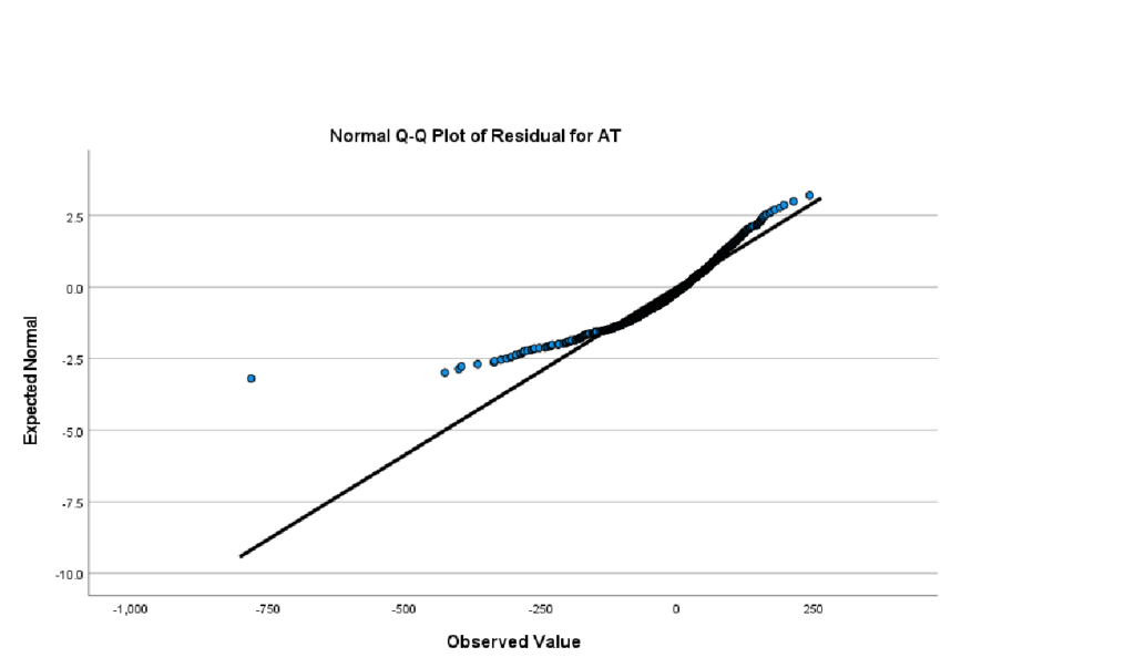
The figure shows a mild violation of normality. But, ANOVA is robust to minor violations.
The second assumption tested in SPSS is homogeneity of variance using Levene’s test:
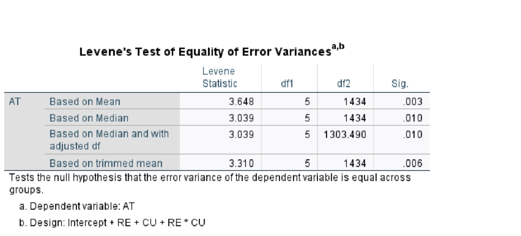
In this case, there is a violation of the assumption (based on mean, Sig. < .05). This means conclusions from ANOVA, especially hypothesis tests and estimation of effects, cannot be relied upon. The first option when a violation of homogeneity of variance occurs is to transform the data. In the alternative, the Kruskal-Wallis test is the non-parametric equivalent of ANOVA. Kruskal-Wallis is one option when the assumption of homogeneity of variance is violated. The Kruskal-Wallis test is robust to violations of this statistical assumption. Researchers report medians and interquartile ranges instead of means and standard deviations when using the Kruskal-Wallis test.
Let’s proceed as if the assumptions were met. We now check our SPSS outputs.
Hypothesis tests
We rely on the Tests of Between-Subjects Effects table (F tests and associated p values [Sig.]) as the most important and most useful table for ANOVA hypothesis tests.
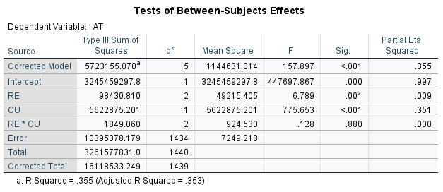
In this case, we see that the p value for region (RE) = .001, which is less than a level of significance of .05. We reject the null and conclude that there is a difference in means among the regions in this example.
The p value for CU < .001. Again, reject the null and conclude there is a difference in mean achievement test scores based on curriculum.
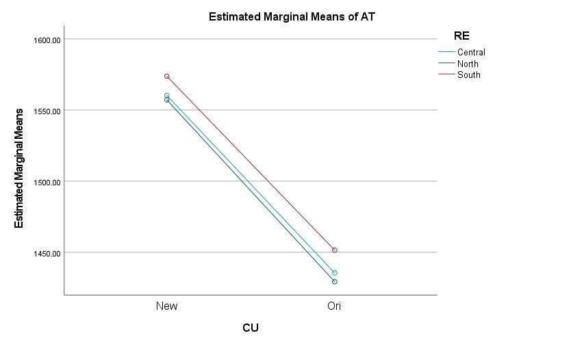
The p value for the interaction between RE and CU = .880. We fail to reject the null hypothesis and conclude there is insufficient evidence that there is a significant interaction. This result is corroborated in the plot of cell means, for which the plots are parallel:
Predictive model of the dependent variable
Having tested the ANOVA hypotheses, and concluding that both region and curriculum are factors with significant influence on achievement test scores, there are questions remaining. One is, how sensitive are scores to the predictors? There are useful tables provided by SPSS, including Descriptive Statistics and Estimated Marginal Means. But, the table most useful for the predictive model is the Parameter Estimates table:
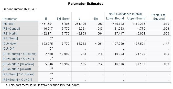
This table shows the effects from each value or level of the predictors. For example, the grand mean of test scores = 1451.504. To predict a value for test scores, we apply estimates of the specific effects, as in this example:
Central region = -16.017
New Curriculum = 122.275
Interaction = 2.558
The predicted value of AT = 1451.504 + (-16.017) + (122.275) + (2.558) = 1560.316
Among the 1440 total records, and 240 for this case (central region, new curriculum), student #352 had an actual score = 1507. The difference between the actual score and the predicted score is the error, or residual = -53.32.
ANOVA produces estimates for each level of each factor (treatment), some of which are zero. Consider the treatments with estimated effects = 0 to be baseline cases. The predicted score for south region and original curriculum = grand mean = 1451.504. Effects of other treatments incrementally increase predicted test score. For example, a student under the new curriculum is predicted to have an increase in test score of 122.275 versus the original curriculum.
Goodness-of-fit
Adjusted R2 = .353: Approximately 35% of the variation in Y is attributed to the model consisting of factors A and B, and their interaction. This may be considered a low goodness-of-fit. There are likely other significant predictors of Y (e.g., family income) that the researcher ought to consider.
A quick review of model-building
We would not have a thorough, complete analysis if we stopped here. A one-time run of ANOVA with predictors is incomplete. Instead, we need to find the best predictive model of the dependent variable, through model-building. I explain this in detail in two other articles on multiple linear regression and two-factor interactions.
The point is, in ANOVA as in regression, we simply cannot make a truthful statement about the influence of any single factor without simultaneously considering all influential factors. These are expressed in a final mathematical model, developed through a rigorous, sequential model-building process:
- Identify candidate predictors.
- Screening: Employ ANOVA model-building to eliminate candidate predictors that are NOT significant.
- Employ purposeful sequential ANOVA (manual stepwise employment of multiple ANOVA runs) to evaluate various combinations of factors and factor interactions.
- Find the best model of predictors and factor interactions.
Final thoughts
Often, in dissertations, theses, and real-world analyses, we are evaluating the influence of multiple factors on some measurable phenomenon. When those factors are numerical or a combination of numerical and categorical, the best tool is multiple regression analysis. When the factors are categorical, the tool is ANOVA.

There are many similarities between regression and ANOVA. Perhaps the most significant is the need to perform a model-building process, purposefully employing sequential ANOVA runs, to find the best combination of factors—the best predictive model.
Doing this correctly, we can report on the sensitivity of the dependent variable to the significant predictors. And, we can use a mathematical model to predict the dependent variable as a function of various treatments—the values or levels of our predictors.
References
Cohen, J. (1988). Statistical power analysis for the behavioral sciences. Hillsdale, New Jersey: Lawrence Erlbaum Associates.
Faul, F., Erdfelder, E., Buchner, A., & Lang, A. G. (2009). Statistical power analyses using G*Power 3.1: Tests for correlation and regression analyses. Behavior Research Methods, 41, 1149-1160.
IBM Corporation. (2020). IBM SPSS Statistics for Windows, Version 27.0. Armonk, NY: IBM Corp.
Levine, D. M., Berenson, M. L., Krehbiel, T. C., & Stephan, D. F. (2011). Statistics for managers using MS Excel. Boston, MA: Prentice Hall/Pearson.
Scale Statistics (2022). Correct for violating the assumption of homogeneity of variance for ANOVA. Retrieved from https://www.scalestatistics.com/kruskal-wallis-and-homogeneity-of-variance.html
Simon, S. (2010). What’s the difference between regression and ANOVA? Retrieved from http://www.pmean.com/08/RegressionAndAnova.html
Warner, R. M. (2013). Applied statistics: From bivariate through multivariate techniques. Los Angeles: Sage.